TRUE and FALSE argument in Vlookup!
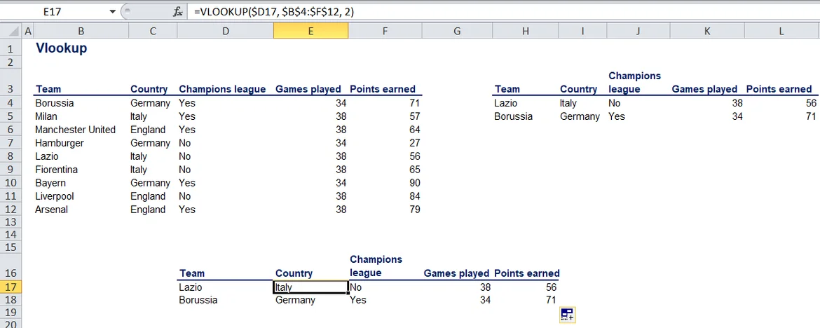
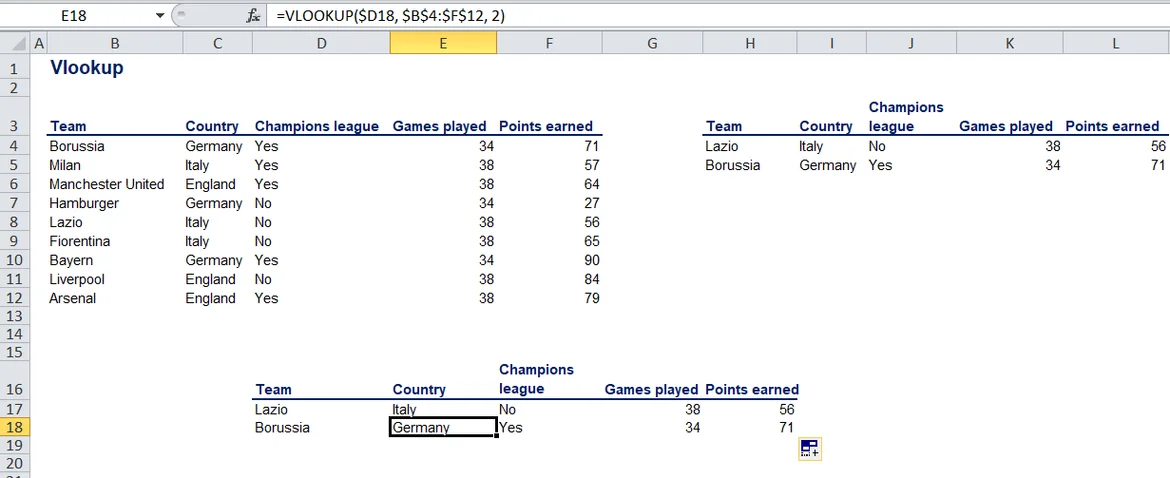
I was solving the Vlookup exercise within the resources. I noticed something - If I do not use the False argument for looking up "Sony" value from the table I get the desired output. But when I copy this formula with proper cell referencing to lookup "Panasonic" value I get an error.
The error is resolved once I pass the False argument.
Why is the case?
And I think the True/False arguments are optional for vlookup formula,  if not please let me know.
Hello,
Good to hear from you.
The TRUE and FALSE arguments are optional, but they are also quite important.
If you select FALSE you are telling Excel that you want it to find an exact match of the value you are looking for.Basically you want to tell Excel that if it doesn't find this exact match you should receive N/A as you did here. The reason why you received N/A in this case is that probably there is blank space in one of the two 'Panasonic' cells. Please take a look. If not, please try to Copy, Paste, Values for both cells. In this way, the formula will work.
If you opt for FALSE in your function, on the other hand, you will tell Excel to find you the closest match to the cell you are looking for. This is very valuable when you want to categorize numbers in bins. In this case, Excel is less likely to give you an N/A error because it doesn't look for a specific value but for a close match.
Best,
Ned
Hi Ned,
The doubt is still not clear.
1. What is meant by blank space in a cell? If it means an empty cell then there are no empty cells in the table.
2. It is clear to me what True and False arguments do. But in the above case I get the desired output when I look for 'Sony' value in the table without True/False arguments and I get an error when I copy-paste or fill the cell below it(shown in screenshot).
3. If I directly use Vlookup formula inside H3 cell without True/False arguments I get the desired output but the same is not true for H4 cell, I get an error.
Hello Aniruddha,
The problem is with your table array
It should be =VLOOKUP(G3,$A$3:$E$8,2,0) and not =VLOOKUP($G3,$A$2:$E$7,2,0)
I hope this helps
Thanks,
What you said worked but I can't figure out what is wrong with my formula:
=VLOOKUP($G3, $A$2:$E$7, 2)
The lookup value is in the first column of the table array so why isn't this working?
Should I be worried about this or not?
This is weird! Here it is working absolutely well without TRUE and FALSE arguments.
I guess it's better I not bother too much about it.


Hi,
If you omit the argument, Excel performs the function as you have added a TRUE argument.
Best,
Ned
If anyone knows why is this happening let me know. Same formula different results.


Hi,
Please check if you have typed Panasonic correctly. Perhaps you have added an extra blank space at the end and you have "Panasonic "? If that's the case Excel is not going to be able to recognize the lookup value.
Best,
Ned
Yes,
I have typed Panasonic correctly