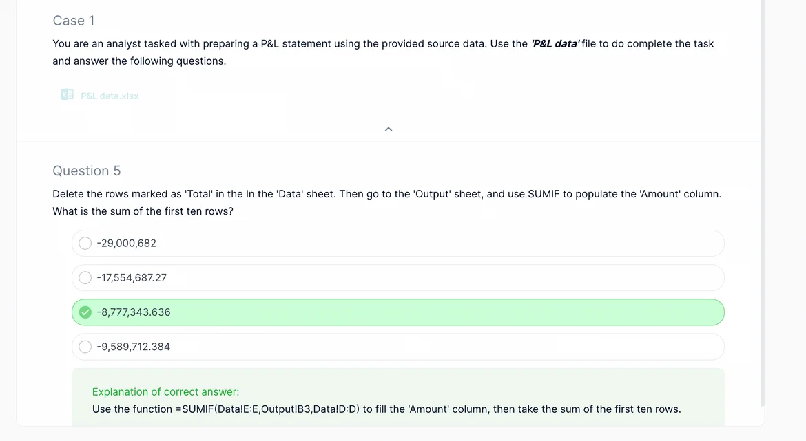
I need help with Question 5 from practice exam 3
Hello, I need help with the SUMIF formula from practice exam 3, I still don't understand why the formula looks like that? Why we put E:E as range and why B3 from output as criteria? are we looking for the amount? How to find the first 10 rows? I am so confused by this results. I applied the formula from the lecture but it not seems working. Can anyone help me solve this problem? Thank you so much! 
Hi Thy,
Apologies for the confusion.
First, you have to delete the 'Total' rows from the 'Data' sheet. Hope this part is clear.
Then, once you have done that you need to create a SUMIF function. It can either take the entire column where you have range and sum range - like in the answer which we have provided - we take the entire column E and the entire column D to perform SUMIF for all rows in the sheet. Alternatively, the function can look like this:
=SUMIF(Data!$E$4:$E$60,Output!B3,Data!$D$4:$D$60)
Hope this helps!
Please let me know if it doesn't.
Thank you!
Exercise#5 is preceded by #1, if you have not completed exercise #1, then the result on the #5 will never match any of the answers. This is the missing step of exercise #5, not mentioned anywhere.


