VLOOKUP and HLOOKUP Examples

VLOOKUP and HLOOKUP are among the most frequently used functions in Excel. They allow users to transfer large quantities of data based on a given criterion.

What are their differences, and when and how do we use each? We demonstrate with practical examples the VLOOKUP and HLOOKUP usage.

Feel free to download VLOOKUP and HLOOKUP practice sheets we’ll use in this article:

HLOOKUP vs VLOOKUP Example

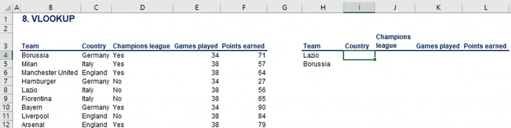
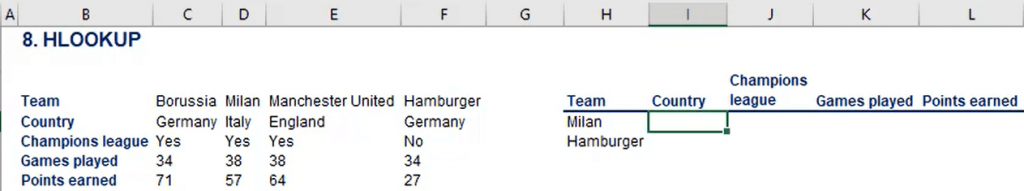
The illustration below presents a worksheet with two similar tables. Both contain football teams’ names and countries and information about the number of games played, points earned, and whether they’ve won the Champions League. The difference is that the table on the right includes only two teams’ names and is otherwise empty.

Our task in this example will be to populate this space using the HLOOKUP and VLOOKUP functions in Excel. First, we’ll use the VLOOKUP formula to find the corresponding fields in the table on the left and populate the table on the right.

What Is a VLOOKUP?

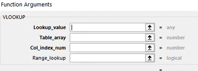
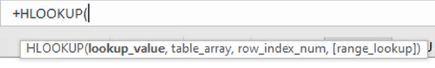
The VLOOKUP (vertical lookup) function searches for a specific value from the first column of a dataset and retrieves the corresponding value from another column. It has four arguments:

1. Lookup value. This is the value we use to search, which serves as a key and makes the connection with the data source. (In this case, the lookup values are Lazio and Fiorentina in cells H4 and H5.)
2. Table array. This source table represents the dataset (data array) to be searched—i.e., the table on the left (above) from which we’ll extract data.
3. Column index number. We extract a value from this column when there’s a match.
4. Range lookup. This feature tells the formula to look for the closest or exact match. This argument can take on two forms: TRUE or FALSE. With TRUE, we say finding the closest match is OK, while FALSE indicates that we want an exact match.

Remember, the first column of the source table must contain the lookup value.

Let’s practice the VLOOKUP using the table with the football teams.

How to Use VLOOKUP

We aim to extract the information related to them from the source table.

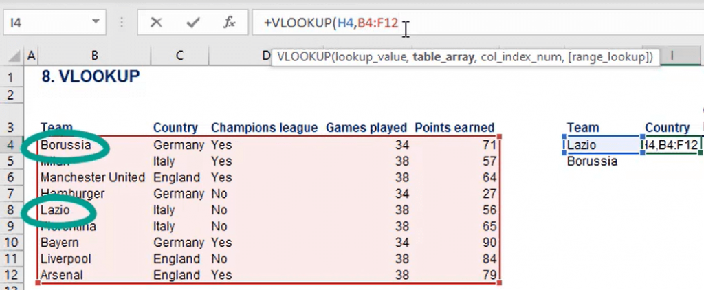
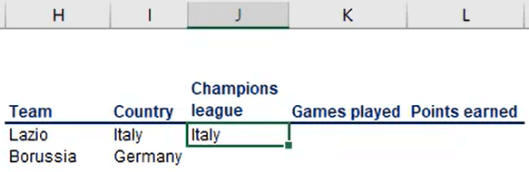
So, click on the first cell from the empty Country column on the right and type +VLOOKUP. Next, select H4 as a lookup value (team Lazio) and the source table where we’ll perform the search (from B4 to F12). Then, Excel will show that the first column of the selected table contains the lookup value Lazio, a necessary condition.

For the third argument of the formula, type ‘2’ because we want to populate the Country column on the right with data from the source table’s second column. The last argument should be FALSE because we need an exact match.

Finally, the VLOOKUP formula should look like this:

=+VLOOKUP(H4,B4:F12,2,FALSE)

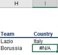
If we’ve done everything right, the function should recognize that we’re looking for Lazio and extract the corresponding value from the source table’s second column (Italy).

Let’s say we want to repeat the same for the next value. We copy and paste the formula in cell I5 next to Borussia. Excel will show an error message indicating that it couldn’t find a matching value in the first column of the source table.

But why?

We can press F2 to see the VLOOKUP function’s arguments and try to identify the mistake. We see that the source table has changed its location. To prevent this from occurring when we move formulas, we must add dollar signs to the references that shouldn’t change:

=+VLOOKUP(H4,$B$4:$F$12,2,FALSE)

If we move the formula to the right, Excel will display the error message again because the lookup value has changed its position. So, we add a dollar sign in front of the column reference to fix the lookup value’s column position:

=+VLOOKUP($H4,$B$4:$F$12,2,FALSE)

Now, our output is ’Italy.’ But this time, we want to obtain data from the Champions League column. So, we also need to change the column index number to 3.

Finally, we can copy the formula for the rest of the table, remembering to change the column index number when we extract from new columns.

Now, let’s see how to use HLOOKUP.

What Is an HLOOKUP?

The HLOOKUP vs VLOOKUP difference is small but significant. The only thing that changes in the formula’s function is the direction. While VLOOKUP searches columns (vertically), HLOOKUP works in rows (horizontally).

Let’s go back to our VLOOKUP and HLOOKUP examples table.

The HLOOKUP function requires the same arguments as VLOOKUP. But the lookup value must be in the first row of the source table, and instead of a column, we have a row index number.

1. Lookup value
2. Table array
3. Row index number
4. Range lookup

How to Use HLOOKUP

First, we type HLOOKUP and select Milan as the lookup value (cell H4). We already know we need to fix the column reference H to block the column movement of our lookup value but allow it to remain flexible vertically.

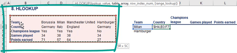
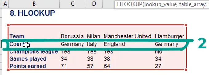
Next, we select the source table and fix all the references to facilitate our work later. The third argument in the HLOOKUP formula is the row from which it should extract a value. Here, we look for ’Country’ (the second row of the source table) and type the number 2.

Finally, we choose FALSE because we need an exact match and close the brackets.

Our final Excel HLOOKPUP function looks like this:

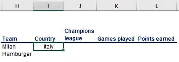
=+HLOOKUP($H4,$B$3:$F$7,2,FALSE)

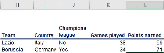
We input it in cell I4 and obtain Italy.

Since we’ve added dollar signs in all the necessary places, we can apply the formula to the rest of the table. We only need to modify the row number we wish to extract data from.

This is the practical application of HLOOKUP and VLOOKUP in Excel.

VLOOKUP and HLOOKUP Examples: Wrap Up

The difference between VLOOKUP and HLOOKUP is that the former searches for values vertically (in columns), while the latter horizontally (in rows). Our tutorial has shown you how to do both.

Download the free spreadsheets above and practice your HLOOKUP and VLOOKUP skills.

Learn to work with other valuable functions, perform multi-layered calculations, create charts, manipulate data, and more with our Introduction to Excel course. Become proficient in Excel to speed up work or increase your hiring probability.