INDEX and MATCH – the Perfect Substitute of VLOOKUP

INDEX and MATCH are two of the most interesting Excel functions. The INDEX function can return an item from a specific position in a list. The MATCH function can return the position of a value in a list. The INDEX / MATCH functions can be used together, for the purpose of extracting data from a table. That combination offers an interesting alternative to VLOOKUP.

---

You can find more about the Lookup functions (VLOOKUP/HLOOKUP) and how to use them in our previous article.

Please feel free to download the spreadsheet files we will use in this article:

---

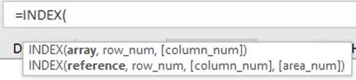
 INDEX is a formula, which returns the value located at a given intersection within an array.

So basically, the INDEX formula needs us to indicate the following:

1. An array where it will function
2. A row number
3. A column number

The formula will go and find the specified row and the specified column within the array and deliver its content.

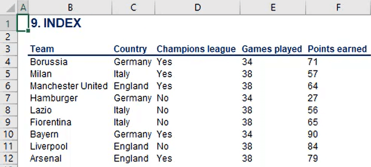
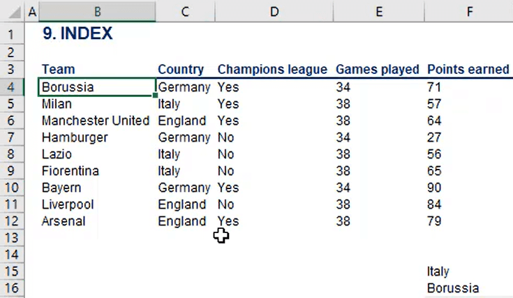
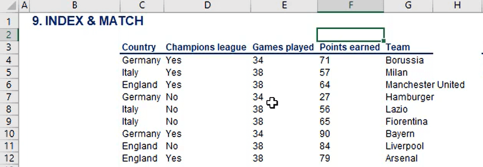
For example, if the array from B4 to C12 is selected in the table, and 5 is chosen as the row argument and 2 as the column argument, “Italy” will be obtained as a result.

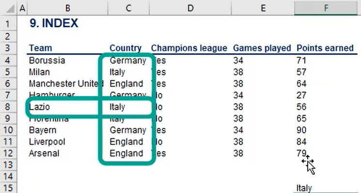
The INDEX function simply delivers the cell which has the coordinates we chose. Within the fifth row and second column of the range we selected lies “Italy”. If those coordinates have been added, the result will be provided.

 The formula should look like this:  

=INDEX(B4:C12,5,2)

Let’s do another try and select the same range – from B4 to C12. This time let us pick 1 as the row argument and again 1 as the column argument. The result will be “Borussia,” given that the value in the first row and first column of the selected range is “Borussia.”

The next function we will look at is MATCH. MATCH returns the relative position of an item within an array.

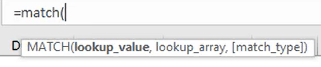
 The MATCH function has 3 arguments:

1. Lookup value
2. Lookup array
3. Logical value

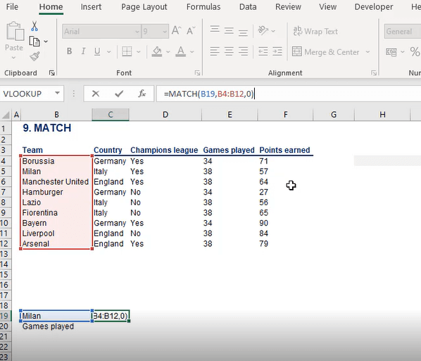
The first argument that needs to be selected is the lookup value – in this example, that will be “Milan,” lying in B19. After that, we need to specify which is the array where the lookup value’s position needs to be found. All teams that lie within the range from B4 to B12 should be selected for that. The third argument is a logical value – “0” or “1,” standing for “an exact MATCH” and “closest MATCH.” Zero will be selected, as an exact MATCH is needed.

 Now the formula is ready, and it should look like this:

=MATCH(B19,B4:B12,0)

The output of the function will be “2,” which represents Milan’s position within the selected array.

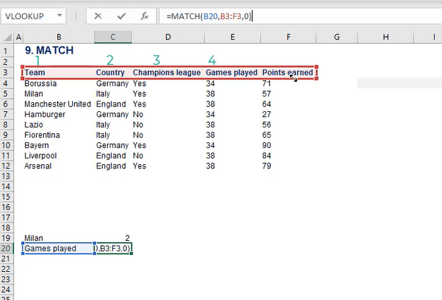
It is important to notice that the formula can be applied vertically. For example, if we go on and look at number of games played within the array from B3 to F3, the result will be four, which is correct as “Games Played” is the fourth column within the array.

Let’s consider the combination of INDEX and MATCH together. This is a pretty powerful tool, often considered superior to VLOOKUP.

It allows users to have a flexible lookup value within the Source table. It is intuitive to combine INDEX and MATCH. The first formula needs as an input relative positions within a range, and the second formula provides that.

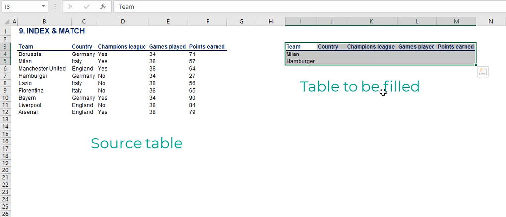
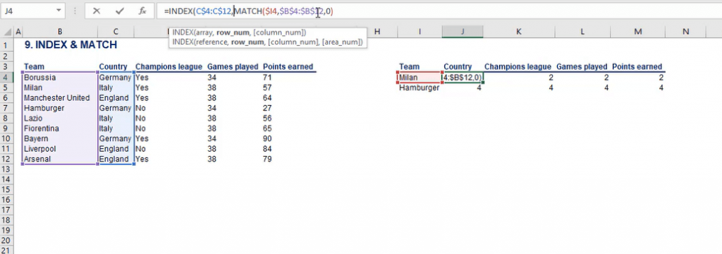
In this picture again we see two tables. The one on the left is our source table and the one on the right needs to be filled.

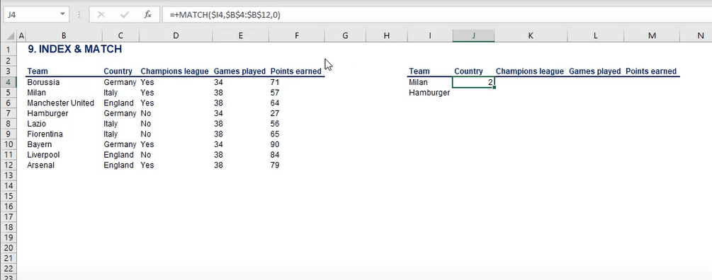
First, the MATCH formula will be applied to each of the blank cells in the table on the right.

So, we have +MATCH, the lookup value is Milan in cell I4. Its column reference has to be fixed, as this will be the lookup value of our table.  Then the cells from B4 to B12 should be selected as a lookup array and fixed after that. We are looking for an exact MATCH so 0 should be typed as the third argument of the formula.

It should look like this:

=MATCH($I4,$B$4:$B$12,0)

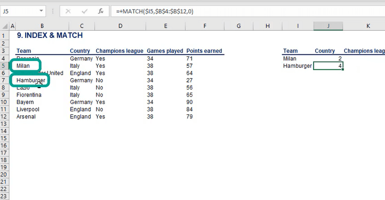
That should be copied on the row below as well. The obtained results are that Milan is in the second position and Hamburger is in the fourth position within the selected array, and this is correct.

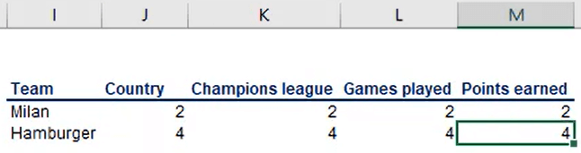
Now, if we copy the two formulas for the rest of the blank cells, we will have the position of the lookup value within the source table, which does not do much work for now.

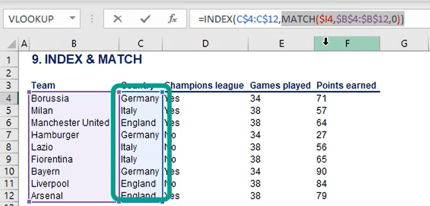
What needs to be done is to type INDEX in front of the MATCH function and add a left parenthesis. INDEX needs an array as a first argument. The array is the range of cells among which the output of the INDEX formula is selected. The cells from C4 to C12 must be selected and their row references should be fixed. Then the parentheses can be closed.

The formula should look like this:

=INDEX(C$4:C$12,MATCH($I4,$B$4:$B$12,0))

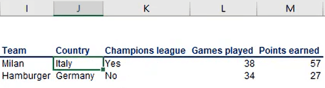
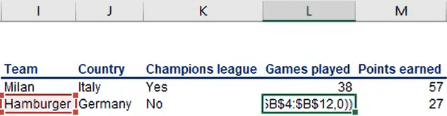
The result we obtained is “Italy”.                                                                                                     

Let’s recap how the two functions work together.

=INDEX(C$4:C$12,MATCH($I4,$B$4:$B$12,0))

The INDEX formula needs as an input the number of the row within a range. And the number we were looking for was found, thanks to the MATCH function. In other words, the MATCH function indicates the position of the result and the INDEX function extracts it.

It is important that the INDEX function’s first argument is the array of the source from which we want to extract the result. The second argument of the INDEX function is the MATCH function, which finds the exact piece of data that we are looking for.

In many cases INDEX, MATCH is superior to VLOOKUP. For example, If the values are cut under the column “Team” within the source table and pasted in Column G, nothing will change with the table on the right.

 This is because the combination of INDEX and MATCH works, even when the lookup value is on the right. If VLOOKUP was used, we would have seen an instant N/A error message. The combination of INDEX and MATCH is great for situations when you have an original source sheet and you do not want to change anything in it and your lookup value is on the right.