What is the Payback Period?
Join over 2 million professionals who advanced their finance careers with 365. Learn from instructors who have worked at Morgan Stanley, HSBC, PwC, and Coca-Cola and master accounting, financial analysis, investment banking, financial modeling, and more.
Start for Free

The Payback Period calculates how long it takes for an organization to get back the funds it originally invested in a project. In other words, it is the time needed for an investment to break-even.
How to calculate the Payback Period
When calculating the Payback period, there are two instances we need to consider relative to a firm’s yearly cash flow.
If a company expects to receive annuities, it calculates the Payback Period by simply taking the amount of the initial outlay and dividing it by the yearly cash flow.1 A firm that invests $100K in a project that yields $20K each year will have a payback period of exactly 5 years.
Other projects, however, do not have fixed cash flows. In this case, one should first calculate the cumulative cash flows, given the expected cash flows. Afterward, they should find the last year in which the cumulative cash flow is still a negative figure.
In practice, firms rarely recover the invested outlay in exactly 3, 5, or 7 years; they would most probably want to as well compute the fraction of the year in which the amount is recouped (i.e. 3.6 years). They can do that through extrapolation, using MS Excel.
Example of Payback Period
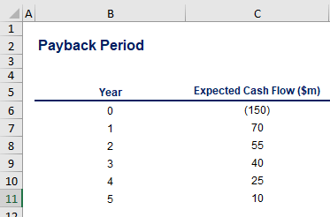
Imagine that you have been assigned to evaluate the economic benefits of a new project. You have estimated the expected cash flows (see below), and the CFO asks you to find out when the investment will pay back in full.
So, you calculate the Payback Period in Excel by using the following steps:
1. Аdd a column with the cumulative cash flows for each period, i.e. the accumulated amounts that are expected throughout the project’s life. The initial investment equals minus $150 million. After the first year, the project pays back $70 million, leaving $80 million to be recovered; year 2 provides yet another $55 million, which makes the cumulative net cash flow go down to minus $25 million, and so on.
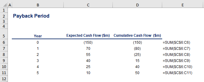
Once you do this for the entire period, you are ready to move on to the next step. A word of caution! Do not forget to ‘freeze’ the first cell in the range and leave the last cell free of anchors before you continue. This would allow you to sum up the accumulated cash flow at each time interval. Use the formulae as presented on the picture above.
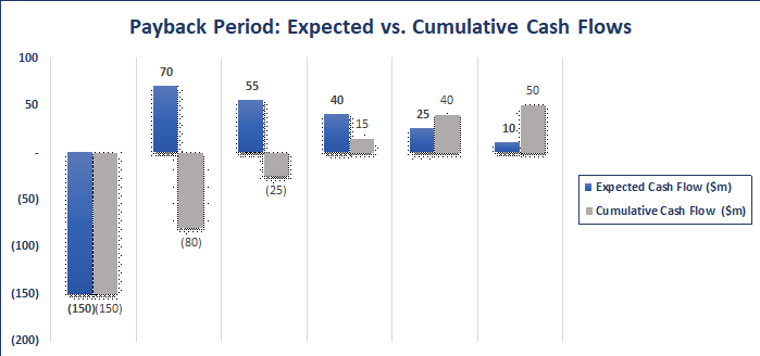
2. Find the last year in which the cumulative cash flow is still a negative figure.
In our example, we establish that the last year in which the cumulative cash flow is still negative is year 2 for which we had forecast a cash inflow of $55 million (see the graph below). That said, the project pays back in full at some point in time between the second and the third year.
3. Estimate the fraction of the year in which the amount is recovered.
At the beginning of the second year, we needed only $25 million until the break-even point. Thus, we divide $25 million by $40 million to approximate the result. In the end, we estimate that it takes 2.63 years for the principal amount to recover (or 2 years and 7.5 months):
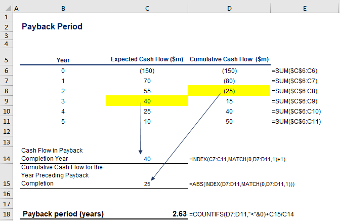
As you can see on the picture above, we use a combination of index and match formulae to find the cash flow in the year we reach the breakeven point (40), and index & match again to find the cumulative cash flow for the year before reaching a breakeven (a negative 25). A countifs formula, counting the periods in which the cumulative cash flow is still negative, completes our model.
Pros and Cons of the Payback Period
The major advantage of the Payback Period lies in its simplicity. Even managers with no financial background comprehend its underlying logic and implications with ease.
The technique also allows us to rank the liquidity of different projects – those with lower payback periods should be perceived as more liquid, and thus more attractive.
Yet, there are a few drawbacks one must take into account when using this model.
First, opportunity cost (or required rate of return) is not considered. Neither is riskiness and the time value of money. Fortunately, another technique, known as the Discounted Payback Period, uses discounted cash flows to adequately address these concerns.
Second, the Payback Period is a measure of payback time, but it is not uncommon for some people to mistakenly take it as a measure of profitability. False interpretation may potentially take investors in the wrong direction.
And third, it omits cash flows that are forecast beyond the payback year. That way, the focus remains on short-term profitability.2 This implies that the technique ignores the later time intervals by relying on the pure Payback Period only. An investment might have considerable cash inflows projected to materialize in the last years of the project’s life. On other occasions, it might turn negative in any year beyond the payback completion year but be left overlooked by the model.
Beyond the Payback Period
The Payback Period is a useful tool in the analysts’ toolbox. Still, a financier should use it in conjunction with other metrics, in order to draw meaningful conclusions as to whether the Payback Period is economically sound or not. Making investment decisions solely based on the time needed for an initial outlay to pay back in full is not a good practice.
To learn more about how to conduct a proper company analysis, read the additional resources we have prepared for you!
If you want an example of a Payback Period in Excel, take a look at our Payback Period Excel template.