Logarithmic (Log) Returns in Finance
Logarithmic (log) returns are a powerful financial tool for analyzing short-term investment performance due to their compounding and time-additive properties. While they offer analytical precision, they’re less intuitive and unsuitable for aggregating returns across multiple assets, making them best for specific modeling scenarios.
Join over 2 million professionals who advanced their finance careers with 365. Learn from instructors who have worked at Morgan Stanley, HSBC, PwC, and Coca-Cola and master accounting, financial analysis, investment banking, financial modeling, and more.
Start for Free
In finance, accurately measuring investment performance is essential for informed decision-making and strategy development. A commonly used metric is the Holding Period Return (HPR), which captures the total return from holding an asset over a specific time frame—a day, a month, or a year. By dividing this time horizon into smaller sub-periods, we gain insights into how returns accumulate over time. As we move toward increasingly smaller intervals—approaching a continuous scale—we arrive at the concept of continuous compounding, which naturally leads us to log returns.

This equation expresses the future FVN of an investment under continuous compounding, where PV is the present value, rs is the continuously compounded rate, and e is the base of the natural logarithm.
Calculating Logarithmic Returns
When these sub-periods are reduced infinitely, we move into continuous compounding. Continuous compounding reflects a situation where returns are reinvested constantly, leading to exponential growth of investments. The formula used to calculate the future value with continuous compounding—when rearranged and simplified—yields what we call the logarithmic return, also known as the continuously compounded return:

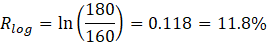
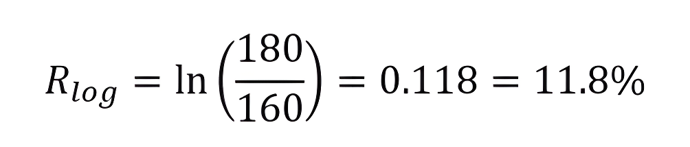
For instance, if shares of Shevon Holdings rise from $160 to $180 over 10 days, the log return is approximately 11.8%.
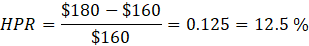
Conversely, this scenario’s regular holding period return (HPR) is about 12.5%, illustrating a difference due to the compounding effect captured by log returns.
Advantages of Logarithmic Returns
► Effect of Compounding
Log returns account for compounding effects, highlighting how investment earnings reinvested in each period generate additional profits. This makes log returns a valuable tool for financial modeling.
► Time-Additivity
Another benefit of log returns is their additive nature over time, simplifying calculations. Consider a scenario where a stock bought for $50 increases to $70 in one year and falls back to $50 the following year. With HPR calculations, you might misleadingly find an average positive return despite no real gain:
- Year 1: +40%
- Year 2: -28.66%
(Average HPR misleadingly suggests gains.)
Logarithmic returns accurately reflect reality:
- Year 1: +18.2%
- Year 2: -18.2%
(The log return averages zero, correctly indicating no overall gain.)
Disadvantages of Logarithmic Returns
Despite their advantages, log returns also come with certain limitations:
► Lack of Intuition
Log returns are less intuitive because real-world investments rarely compound continuously. Therefore, they’re typically used only for short intervals (usually daily).
► Not Asset-Additive
Log returns are useful for analyzing the return of a single asset over time—particularly when considering continuous compounding. The formula for log return is:
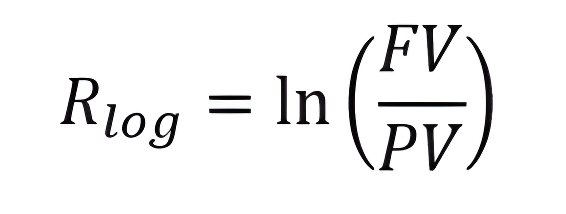
For example, if an asset grows from $160 to $180, the log return is:
Let’s say you hold a portfolio with:
- Amazon: 60% weight, 6% return (HPR)
- Facebook: 40% weight, 8% return (HPR)
To calculate the total portfolio return using HPR, you can simply apply a weighted average:

This result accurately reflects the return of the portfolio over the holding period.
Practical Example
Imagine investing equally ($1,000 each) in five different stocks:
- Stock A: +40%
- Stock B: +10%
- Stock C: +20%
- Stock D: +25%
- Stock E: -30%
Using the SUMPRODUCT function in Excel to calculate the holding period returns, the portfolio return accurately comes out as 13%. This is validated by the final portfolio value calculation ($5,650 final vs $5,000 initial investment).
Log returns, however, result in an incorrect portfolio return of 9.6%. This discrepancy occurs because log returns assume continuous compounding, which is inappropriate when combining simultaneous returns from multiple assets.
Balancing Precision and Practicality in Log Return Analysis
Log returns offer distinct analytical advantages, primarily due to their compounding nature and time-additivity. But their complexity and limitations in asset aggregation mean they are typically suited only to short-term financial modeling scenarios. Holding period returns remain the preferred, practical choice for portfolio evaluations and longer investment horizons.
If you’re looking to master when and how to apply log returns effectively across different financial contexts, the 365 Financial Analyst platform offers structured guidance and hands-on learning.